Convex Restriction
Motivation
Convex restriction was one of my favorite results from my Ph.D. studies, and this page is my attempt to explain the idea as concisely as possible.
One of the fundamental problems in nonlinear systems is solvability:
Under what conditions can we solve a system of nonlinear equations?
Consider the quadratic equation $ax^2+bx+c=0$. From the quadratic formula, we know that a real solution exists if and only if
\[b^2-4ac \geq 0.\]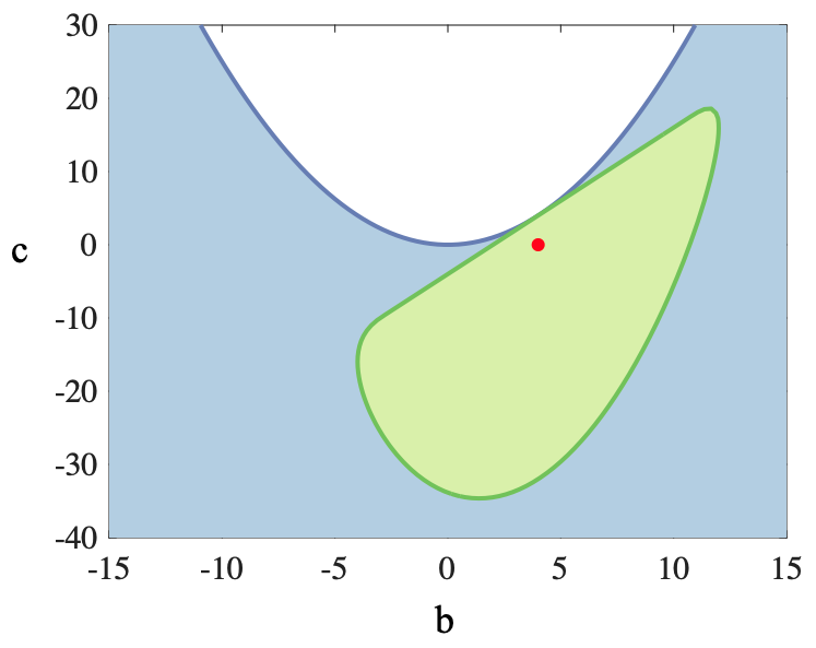
Figure 1. The solvability condition $b^2-4ac \geq 0$ with $a=1$ is shown in blue. An example of a convex restriction is shown in green.
We can derive this condition for simple systems such as quadratic equations, but nonlinear systems generally do not have closed-form solutions. Consider the more general system
\[\begin{aligned} f(x,u) &= 0, \\ h(x,u) &\leq 0, \end{aligned}\]where $x\in\mathbb{R}^n$ represents implicit variables defined through $f:\mathbb{R}^n\times\mathbb{R}^m\to\mathbb{R}^n$, $u\in\mathbb{R}^m$ represents explicit variables, and $h:\mathbb{R}^n\times\mathbb{R}^m\to\mathbb{R}^p$. In the quadratic example, we would define the decision parameter as $u=[a,\,b,\,c]$. Convex restriction seeks a tractable sufficient condition: a convex set of parameters for which a feasible solution is guaranteed to exist.
Inner and outer approximations
Suppose $\mathcal{F}=\lbrace u\,\vert\,\exists x,\; f(x,u)=0,\;h(x,u)\leq 0 \rbrace$ denotes the true feasible set. A convex relaxation constructs a convex outer approximation $\mathcal{F}_{\mathtt{RELAXATION}}$ such that
\[\mathcal{F} \subseteq \mathcal{F}_{\mathtt{RELAXATION}}.\]Outer approximations are useful for computing bounds. For example, solving a minimization problem with a convex relaxation gives a lower bound on the optimal objective value. However, the solution may not be feasible for the original problem.
A convex restriction constructs a convex inner approximation $\mathcal{F}_{\mathtt{RESTRICTION}}$ such that
\[\mathcal{F}_{\mathtt{RESTRICTION}} \subseteq \mathcal{F}.\]Every point in the restriction is therefore feasible for the original problem. Solving a minimization problem with a convex restriction gives an upper bound on the optimal objective value. We can also view a restriction as a robustness certificate against uncertainty. The tradeoff is conservatism: the restriction may exclude feasible points.
Inequality constraints
For a problem with only inequality constraints,
\[h(x) \leq 0,\]we can simply define
\[\mathcal{F}_{\mathtt{RESTRICTION}}=\lbrace x\,\vert\;h^u(x)\leq 0 \rbrace,\] \[\mathcal{F}_{\mathtt{RELAXATION}}=\lbrace x\,\vert\;h^\ell(x)\leq 0 \rbrace,\]where $h^u(x)$ and $h^\ell(x)$ are convex functions such that $h^\ell(x)\leq h(x)\leq h^u(x)$.
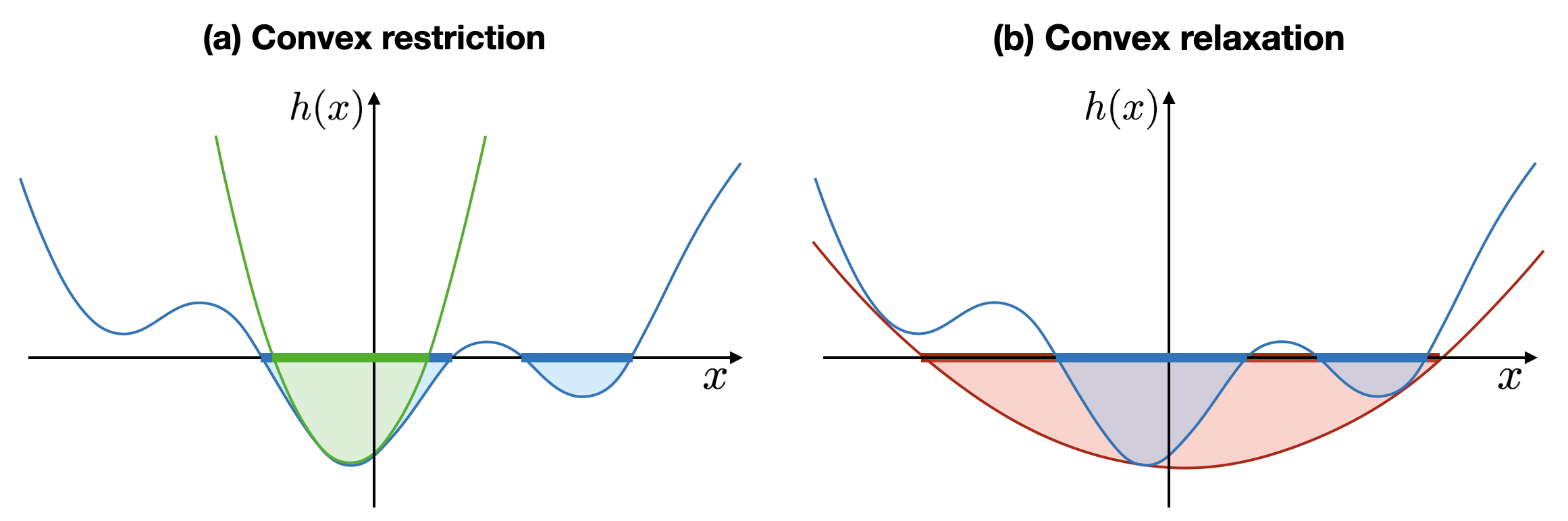
Figure 2. The left figure shows a convex restriction using the convex upper bound $h^u$ in green, and the right figure shows a convex relaxation using the convex lower bound $h^\ell$ in red.
Equality constraints
Equality constraints are more subtle. We first rewrite the equality constraint
\[f(x,u)=0\]in the fixed-point form $x=T_u(x)$ using a nonsingular nominal Jacobian $J$:
\[x=-J^{-1}\bigl(f(x,u)-Jx\bigr)\]where $J$ is the Jacobian of $f$ with respect to $x$ evaluated at a nominal point. This Newton-like preconditioning is useful because Brouwer’s fixed-point theorem provides a way to guarantee feasibility.
Brouwer’s fixed-point theorem. Let $\mathcal{P}\subset\mathbb{R}^n$ be nonempty, compact, and convex. If $T:\mathcal{P}\to\mathcal{P}$ is continuous, then there exists an $x^\star\in\mathcal{P}$ such that $T(x^\star)=x^\star$.
Brouwer’s theorem gives an abstract existence condition, but it does not directly provide inequalities that we can verify or optimize over in practice. To obtain such analytical conditions, we parameterize the box $\mathcal{P}(x^u,x^\ell)=\lbrace x\mid x^\ell\leq x\leq x^u\rbrace$ and search for bounds $x^u$ and $x^\ell$ that certify solvability. We then introduce convex upper and concave lower envelopes to bound the nonlinearity componentwise:
\[f^\ell(x,u) \leq f(x,u) \leq f^u(x,u),\]where each component of $f^u$ is convex and each component of $f^\ell$ is concave. This is the opposite of the concave upper and convex lower envelopes (e.g., McCormick envelopes) used in convex relaxation.
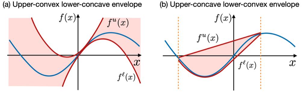
Figure 3. Convex upper and concave lower envelopes used in a convex restriction (left), compared with concave upper and convex lower envelopes used in a convex relaxation (right).
We can now state the main convex-restriction result. The theorem works by constructing a box that is invariant under the fixed-point map. The convex and concave envelopes bound the nonlinear residual throughout the box using conditions checked only at its vertices. If the resulting image remains inside the box, Brouwer’s fixed-point theorem guarantees a fixed point—and therefore a solution to the original nonlinear equations.
Theorem (Convex Restriction). Assume that $f$ and $h$ are continuous and that $J$ is a fixed nonsingular Jacobian. Suppose that, for a given $u$, there exist $(x^u,x^\ell,g^u,g^\ell)$ with $x^\ell\leq x^u$ such that
\[\begin{aligned} &-[J^{-1}]^-g^u-[J^{-1}]^+g^\ell\leq x^u, \\ &-[J^{-1}]^+g^u-[J^{-1}]^-g^\ell\geq x^\ell, \\ &g^u\geq f^u(x,u)-Jx,\quad &\forall\, x\in\lbrace x\mid x_i\in\lbrace x_i^\ell,x_i^u\rbrace,\,\forall i\rbrace \\ &g^\ell\leq f^\ell(x,u)-Jx,\quad &\forall\, x\in\lbrace x\mid x_i\in\lbrace x_i^\ell,x_i^u\rbrace,\,\forall i\rbrace \\ &h^u(x,u)\leq 0,\quad &\forall\, x\in\lbrace x\mid x_i\in\lbrace x_i^\ell,x_i^u\rbrace,\,\forall i\rbrace. \end{aligned}\]where the entrywise positive and negative parts of $J^{-1}$ are defined by
\[([J^{-1}]^+)_{ij}=\max\lbrace (J^{-1})_{ij},0\rbrace, \qquad ([J^{-1}]^-)_{ij}=\min\lbrace (J^{-1})_{ij},0\rbrace.\]The functions $f^u$ and $h^u$ are convex upper bounds, and $f^\ell$ is a concave lower bound. All vector inequalities are interpreted componentwise. Then, for the same $u$, there exists an $x$ such that $f(x,u)=0$ and $h(x,u)\leq 0$.
Proof. Define $g(x,u)=f(x,u)-Jx$ and denote the vertices of $\mathcal{P}(x^u,x^\ell)$ by
\[\operatorname{vert}(\mathcal P)=\lbrace x\mid x_i\in\lbrace x_i^\ell,x_i^u\rbrace,\ \forall i\rbrace.\]Because $f^u(x,u)-Jx$ is componentwise convex in $x$, its maximum over the box is attained at a vertex. Thus, for every $x\in\mathcal P$,
\[g(x,u)\leq f^u(x,u)-Jx \leq \max_{v\in\operatorname{vert}(\mathcal P)}\bigl(f^u(v,u)-Jv\bigr) \leq g^u.\]Similarly, because $f^\ell(x,u)-Jx$ is componentwise concave, its minimum over the box is attained at a vertex, so $g(x,u)\geq g^\ell$ throughout $\mathcal P$. Hence $g^\ell\leq g(x,u)\leq g^u$, and interval arithmetic gives
\[x^\ell \leq -[J^{-1}]^+g^u-[J^{-1}]^-g^\ell \leq -J^{-1}g(x,u) \leq -[J^{-1}]^-g^u-[J^{-1}]^+g^\ell \leq x^u.\]Therefore, the continuous map $T_u(x)=-J^{-1}(f(x,u)-Jx)$ maps the nonempty, compact, convex box $\mathcal P$ into itself. Brouwer’s fixed-point theorem guarantees an $x^\star\in\mathcal P$ satisfying
\[x^\star=-J^{-1}\bigl(f(x^\star,u)-Jx^\star\bigr).\]Multiplying by $J$ shows that $f(x^\star,u)=0$. Moreover, componentwise,
\[\max_{x\in\mathcal{P}}h(x,u) \leq \max_{x\in\mathcal{P}}h^u(x,u) \leq \max_{v\in\operatorname{vert}(\mathcal P)}h^u(v,u) \leq 0,\]so the solution to $f(x,u)=0$ also satisfies the inequality constraint $h(x,u)\leq 0$. $\square$
Because the envelopes are jointly convex or concave in $(x,u)$, and each vertex is an affine function of $(x^\ell,x^u)$, these conditions define a convex set. Its projection onto $u$ is therefore a convex restriction of the feasible parameter set.
Figure 1 illustrates this construction for a quadratic equation.
At first glance, the number of constraints appears to grow exponentially with the problem size: a box in $\mathbb R^n$ has $2^n$ vertices. In many applications, however, the nonlinearity in $f$ is sparse, and each residual depends on only a few entries of $x$. For example, a single-layer neural network can be lifted as
\[u=\operatorname{ReLU}(Wx_{1:N}) \quad\Longleftrightarrow\quad u=\operatorname{ReLU}(x_{N+1:M}), \qquad x_{N+1:M}=Wx_{1:N}.\]Each nonlinear residual $u_i-\operatorname{ReLU}(x_{N+i})=0$ depends on only one implicit variable, $x_{N+i}$. Its envelope therefore needs to be checked at only $2$ local vertices, rather than at all $2^M$ vertices of the lifted box.
Further reading
The initial idea for convex restriction was proposed in the following paper.
- Dongchan Lee, Hung D. Nguyen, Krishnamurthy Dvijotham, and Konstantin Turitsyn, “Convex Restriction of Power Flow Feasibility Sets.” arXiv
You can also find more results and applications in electric power systems, robotics, and machine learning in my thesis.
- “Robustness Verification and Optimization of Nonlinear Systems.” thesis